When it comes to market timing there are endless options to choose from. Even those who are inclined to trade based upon fundamentals will often use some form of trend validation using their favourite technical approach. There is certainly no shortage of literature available on the topic and we would encourage all to enhance their understanding by checking out the extensive resources available online. Traders may often jump from one indicator to another in a quest to find the optimal timing tool but, in my experience, it is better to choose very few, understand their behaviour, and act upon your knowledge base to improve timing skills. Let’s start by have a brief look at what some of the options are.
Oscillators for extremes
These are standalone mathematically generated formulas which can visually represent the performance of a security and will often have a maximum and minimum value, though not always e.g. a minimum value of 0 and a maximum value of 100. Again, there is too much information available on this subject to explore here but, for the purpose of illustration and simplicity, I will mention 2 of the most popular.
Firstly, the RSI (Relative Strength Index) – This is essentially an indicator which compares average gains against average losses over a fixed period (Usually 14 days or bars). With a range of 0 to 100, the general wisdom is that a reading above 70 represents an ‘overbought’ situation for the price data applied, and below 30 equals ‘oversold’. Like many static indicators, there are times where this works very well and others where quite the opposite approach would work better.
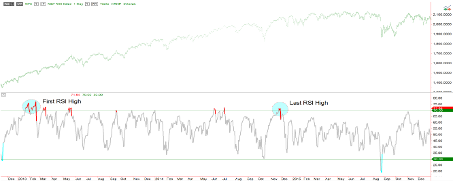
The chart below shows the RSI for the S&P 500 index from 2013 through 2015. From this graph, it is clear to see that using the 70 / 30 extremes as specific points to sell or buy would have resulted in some very poor trades. The first ‘overbought’ point was at an index level of ~1,500 and the final point registered at ~2,000 > 30% higher. Numerous such extreme levels occurred several times in between, providing what are effectively false signals which might encourage some to sell long positions too early, or indeed short with the expectation of lower levels ahead. On a standalone basis, this highlights the challenge of using such rangebound oscillators as timing points. In this basic format, they will tend to work best in range bound markets.
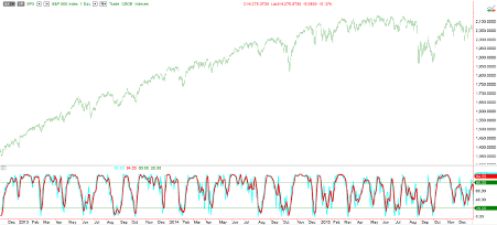
Another similar style oscillator with multiple variations is the Stochastic indicator. In its most simple form (FastK), it can be considered as a location reference type indicator. It looks at the highest and lowest points over a look back period, and simply references, in a percentage format, the current location of the price versus the extremes. For example, if the highest stock price in the past x days is 100, the lowest price is 50, and the current price is 75 (directly in the middle of the extremes), then the indicator will register 50 (%) as it is precisely halfway between the top and the bottom.
The indicator has a ‘smoothed’ version (FastD) too, which is effectively an average of the ‘FastK.’ Smoothing will ordinarily be a simple moving average of the last few data points. However, as will be discussed later, such smoothing can have the drawback of delayed signalling in the form of slower reaction times for changes in trend. The graph below shows the Stochastic Oscillator covering the same data as the above graph for basic comparison purposes.
To conclude, there are many oscillators beyond the scope of this very brief introduction. They will often be used to signal extreme points where some type of price reversion may occur. From the simple example above, as standalone indicators, there are obvious problems using these within strong trends but, as you will see later, they can have their uses, particularly when complimenting trending methodologies which have different characteristics.